Download the file npivfe containing an R file with all functions needed to apply the approach described in the paper as well as a readme file providing a description of the functions.
Model description
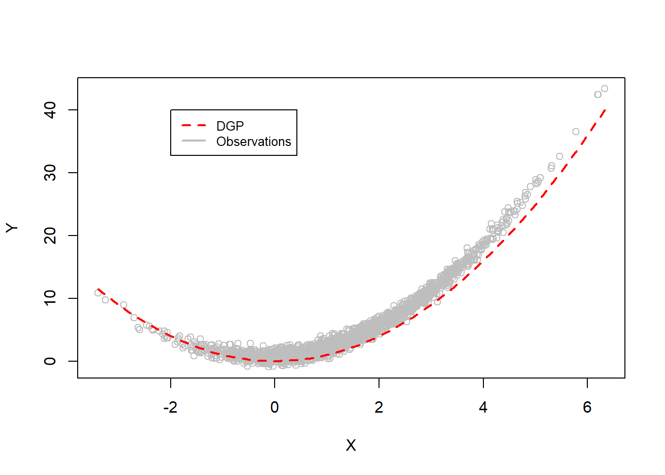
Below we generate data of the two-way fixed effects panel model, given by \[ Y_{it} = \varphi(X_{it}) + \xi_i + \delta_t + U_{it},\] where \(X_{it}\) denotes the endogenous dependent variable that is correlated with both the unobserved individual and temporal fixed effects, \(\xi_i\) and \(\delta_t\), and with the error term \(U_{it}\). Further, we generate a valid instrument \(Z_{it}\), satisfying \[
E(U_{it} | Z_{it}) = 0 \hspace{4mm} \text{and} \hspace{4mm} cor(X_{it},Z_{it}) \neq 0.
\] Note that to stay consistent with the variable convention used in the code, the notation used here changes slightly w.r.t. the one presented in paper. More precisely, while in the paper \(Z_{it}\) and \(W_{it}\) denote the explanatory and the instrumental variable, in the code these variables refer to x and z, respectively.
Data generating process
library(knitr)library(latex2exp)set.seed(49)# Generate panel structure N =100T =20NT = N*Tiota_T =rep(1, T)iota_N =rep(1, N)trend_T =c(1:T)ind_N =c(1:N)col_T = iota_N %x% trend_T col_N = ind_N %x% iota_T # Parts of the DGP in Racine (2019, p. 288) # Correlation parameters rho.xz =0.2rho.ux =0.8sigma.u =0.05# DGP of the quadratic model dgp =function(x){x^2}# Generate endogeneity in x v1 =rnorm(NT, 0, 0.8)v2 =rnorm(NT, 0, 0.15)eps =rnorm(NT, 0, sigma.u)u = rho.ux*v1 + eps # Individual fixed effectsxi_i =runif(N, 0, 1.5)xi_i =as.matrix( xi_i %x% iota_T )# Time fixed effects delta_t =runif(T, 0, 1.7)delta_t =as.matrix( rep( delta_t, N ) )# Explanatory variable needs to be correlated with# the error term as well as with the# individual and temporal effects# Generate "auxiliary" explanatory variablex =matrix( NT, nrow = NT, ncol =1 )# Correlation with individual and temporal effectsfor(i in1:NT){ x[i,1] =rnorm( 1, mean = (xi_i[i] + delta_t[i]), sd =1 ) }# Auxiliary variable used to introduce correlation # between the instrument and the explanatory variablez = rho.xz*x + v2# Generate explanatory variable also correlated# with error term (i.e. E(u*x) != 0)x = x + v1# Dependent variable y =as.matrix( dgp(x=x) ) + xi_i + delta_t + u # Plot the data points along with the true DGPplot( x, y,pch =21, col ="grey", ylab ="Y", xlab ="X" ,main ="")curve( dgp(x),col="red", add=TRUE, lty =2, lwd =2)legend( -2, 40, legend =c("DGP", "Observations"), col =c("red", "grey"),lty =c(2, 1),lwd =c(2, 2),cex =0.8)
Covariance matrix of observables and unobservables
\(x_{it}\)
\(z_{it}\)
\(\xi_i\)
\(\delta_t\)
\(u_{it}\)
\(x_{it}\)
0.27
0.19
0.25
0.52
\(z_{it}\)
0.04
0.05
0
\(\xi_i\)
0
-0.01
\(\delta_t\)
0.01
\(u_{it}\)
To further investigate the data you might assemble the observable variables with the individual and time identifiers:
Data =data.frame( cbind( col_N, col_T, y, x, z ) )colnames( Data ) <-c( "col_N", "col_T", "y", "x", "z" )
Estimation
Load the functions needed for the nonparametric instrumental estimator with two-way fixed effects. (Download above the file npivfe.R containing the functions.)
source(".../npivfe.R")
Use the function npregivfe provided in the package to estimate the conditional mean function \(\varphi\).
Note that the estimation routine is very time intensive as it involves several numerical optimizations to obtain optimal bandwidths as well as several iterations of the Landweber-Fridman regularization procedure. However, I’m sure that the way I coded the estimator can be improved significantly to reduce the run time.
res.npivfe =npregivfe( y = y,x = x,z = z, c =0.5, tol =1, N = N,T = T, max.iter =100,bw_method ="optimal",effects ="indiv-time",type ="ll" )
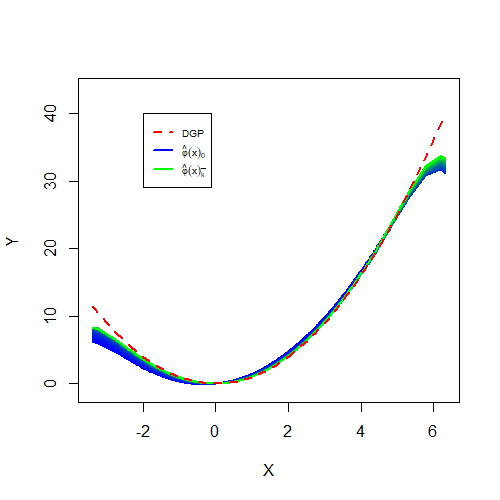
Investigate the regularized solution path:
library(latex2exp)library(colorRamps)# (NT x K) matrix, with K the total number of iterations# within the Landweber-Fridman estimation procedure. phi_k_mat = res.npivfe[[1]]# Total number of iterationsk_bar =ncol( phi_k_mat ) # Final point-wise estimates of the function of interestfit.npivfe = phi_k_mat[, k_bar] # Plot the initial guess phi_0plot( x[order(x)], phi_k_mat[, 1][order(x)],col =blue2green(k_bar)[1],type ="l",lwd =2,ylim =range(y),ylab ="Y", xlab ="X", main ="" ) # Plot all successive estimates phi_k, k=1,...,k_barfor(k in1:k_bar){lines( x[order(x)], phi_k_mat[, k][order(x)], type ="l",lwd =2, col =blue2green(k_bar)[k] )}# Add the true curve curve( dgp, min(x), max(x),add =TRUE, col ="red", lwd =2, lty =2)legend( -2, 40, legend =c("DGP", TeX( '$\\hat{\\varphi}(x)_{0}$'), TeX('$\\hat{\\varphi}(x)_{\\bar{k}}$')), col =c("red",blue2green(k_bar)[1], blue2green(k_bar)[k_bar]),lty =c(2, 1, 1),lwd =c(2, 1, 1),cex =0.65)
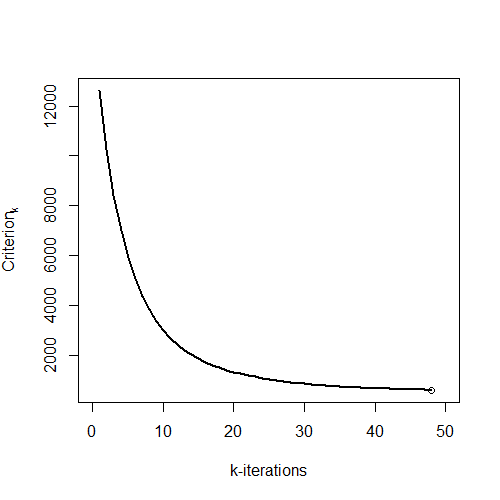
Investigate the evolution of the stopping criterion. Note that the number of iterations of the Landweber-Fridman procedure not only vary when changing the constant c but also for some numerical reasons (bandwidths selection). Even though I here also specified c = 0.5, the number of iterations is slightly higher, given by 48 (44 in the paper).
# Store the values of the stopping criterionval_crit_k = res.npivfe[[2]]# Plot the stopping criterion plot( 1:k_bar, val_crit_k, type ="l", col ="black",lwd =2, main ="", xlab ="k-iterations",ylab=TeX('$Criterion_k $'))points( k_bar, val_crit_k[k_bar] )
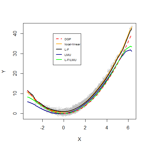
Comparison with other estimators
1.Local-linear kernel regression (LL)
Use the functions npregbw and npreg from the np package to estimate the model by a nonparametric local-linear kernel regression.
First, use the function LMU.CVCMB from the provided package to obtain optimal bandwidths, using leave-one-out conditional mean based cross-validation (CVCMB). Second, use the function LMU.estimator (Lee et al. 2019) with the previously obtained bandwidths to estimate the function of interest.
3.Nonparametric IV using the Landweber-Fridman regularization (L-F)
Use the function npregiv2 from the provided package to estimate the model by nonparametric IV regression (without fixed effects) applying the Landweber-Fridman (L-F) regularization. Note that the function relies on the np package (as it calls the functions npreg and npregbw) and produces very similar results compared to the np::npregiv function (also see Florens et al. 2018).
# Nonparametric IV (without fixed effects)res.npivf2 =npregivf2( y = y,z = x, w = z, c =0.5,tol=1,max.iter =100,bw_method ="optimal" )# Obtain final estimates by selecting the last column (last iteration)fit.npivf2 = res.npivf2[[1]][, ncol( res.npivf2[[1]] ) ]
Plot the results to compare the different estimators.
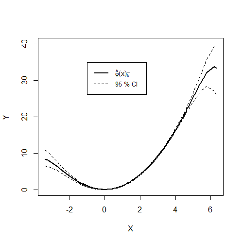
As proposed in the paper, bootstrapped confidence intervals can be obtained by the application of the wild residual block bootstrap following Malikov et al. (2020) and Azomahou et al. (2006). See Appendix B in the paper for more details. The chunk code provided below shows how the estimates were obtained. Note again that the estimation routine is very time intensive. Hence, parallelizing and/or using more computers (as I did) would be useful speed up the routine.
# Use bandwidths from initial estimation of the conditional mean. bws = res.npivfe[[3]]# Compute residuals u_hat v_hat = y - fit.npivfe # Center residuals u_hatv_hat_c =as.numeric(scale(v_hat, center =TRUE))# Create empty lists to store bootstrap estimatesphi_hat_boot_list <-list()# Bootstrap iterations B =400for(b in1:B){# Generate bootstrap weights # each individual i keeps its weight for all t b_i =sample( x =c( (1+sqrt(5))/2, (1-sqrt(5))/2 ), size = N, prob =c( ( sqrt( 5 ) -1 ) / ( 2*sqrt( 5 ) ), ( sqrt( 5 )+1 ) / ( 2*sqrt( 5 ) ) ),replace =TRUE )# Generate new disturbances v_hat_b = (b_i %x% iota_T) * v_hat_c# Generate new outcome variable y_b = phi_hat + v_hat_b# Re-estimate phi_hat using y_b res.npivfe_b =npregivfe( y = y_b, x = x, z = z, N = N, T = T,bw_method ="plug_in", effects ="indiv-time", type ="ll", c =0.5,tol =1, bws = bws,max.iter =100) phi_hat_b = res.npivfe_b[[1]][, ncol( res.npivfe_b[[1]] ) ] phi_hat_boot_list[[b]] <- phi_hat_b}# Bind the results in a (NT x B) matrix. phi_boot =do.call( cbind, phi_hat_boot_list )# Compute the point-wise 95% confidence intervals phi_025 =apply( phi_boot, 1, quantile, probs=0.025 )phi_975 =apply( phi_boot, 1, quantile, probs=0.975 )# Plot the estimates along with the confidence intervals plot( x[order(x)], fit.npivfe[order(x)],ylim =c(0, 40),type ="l",lty =1,lwd =2,ylab ="Y",xlab ="X",main ="")lines( x[order(x)], phi_025[order(x)],lty =2, col ="black")lines( x[order(x)], phi_975[order(x)],lty =2,col ="black")legend( -1, 35, legend =c(TeX( '$\\hat{\\varphi}(x)_{\\bar{k}}$'), "95 % CI"), col =c("black", "black"),lty =c(1, 2, 2), lwd =c(2, 1, 1),cex =0.8 )
Monte Carlo simulation
Lastly, as shown in the paper, a Monte Carlo simulation demonstrates the finite sample properties of the proposed estimator in comparison with other nonparametric estimators, such as those already presented above (i.e. the LL, LMU, and the L-F estimator). The code below shows how the results were obtained. Running the code, however, is very time intensive, which unfortunately renders the reproduction of the results very costly.
Following Lee et al. (2020), the Monte Carlo simulation is performed for four different data sets with \(N\in \{50,100\}\) and \(T\in\{10,20\}\). Each of the estimator is applied on each data set 400 times. To reduce run time, this is done by fixing bandwidths to the ones obtained from the first iteration. Subsequently, the Root Mean Squared Error (RMSE) and the Integrated Mean Absolute Error (IMAE) are computed.
The function dgpivfe provided in the package allows to generate the above described data by specifying the length of the individual and time dimension, N and T, yielding a data.table object that contains the observables y, x, and z.
The table tab.MC provides the results of the Monte Carlo simulation as shown below, where the columns 3 to 6 and 7 to 10 refer to the RMSE and the IMAE, respectively.
\(N\)
\(T\)
L-F/LMU
L-F
LMU
LL
L-F/LMU
L-F
LMU
LL
50
10
1.041
1.664
1.501
1.793
0.350
1.606
0.781
1.675
50
20
0.309
1.660
0.894
1.797
0.123
1.604
0.760
1.678
100
10
0.822
1.670
1.258
1.778
0.250
1.609
0.865
1.660
100
20
0.524
1.663
0.915
1.786
0.116
1.608
0.717
1.668
References
Azomahou, T., Laisney, F., & Van, P. N. (2006). Economic development and CO2 emissions: A nonparametric panel approach. Journal of Public Economics, 90(6-7), 1347-1363.
Florens, J. P., Racine, J. S., & Centorrino, S. (2018). Nonparametric instrumental variable derivative estimation. Journal of Nonparametric Statistics, 30(2), 368-391.
Lee, Y., Mukherjee, D., & Ullah, A. (2019). Nonparametric estimation of the marginal effect in fixed-effect panel data models. Journal of Multivariate Analysis, 171, 53-67.
Malikov, E., Zhao, S., & Kumbhakar, S. C. (2020). Estimation of firm‐level productivity in the presence of exports: Evidence from China’s manufacturing. Journal of Applied Econometrics, 35(4), 457-480.
Racine, J. S. (2019). An introduction to the advanced theory of nonparametric econometrics: A replicable approach using R. Cambridge University Press.